Qualitative Bayes' theorem

Bayes' theorem's concepts can be applied using qualitative methods. First one must commit to the pretest probability – how likely the diagnosis is from the start. This probability is expressed categorically – very unlikely (less likely than 10%), unlikely (between 10% and 33%), uncertain (between 34% and 66%), likely (between 67% and 90%) or very likely (more likely than 90%) (table 1).

If the initial assessment is very unlikely or very likely, then in most cases it is not worth further testing according to Bayes' theorem – the results would either confirm what is already near certain or it would minimally move the post-test probability in the opposite direction. Either way, the clinician would not normally take additional actions. There are at least two situations where it is still important to proceed with further testing. First, if the diagnosis is very unlikely but needs to be ruled out with more certainty, as in a very dangerous disease, the clinician may want to proceed with testing. For example, at what probability is the clinician willing to send a patient home in whom a diagnosis of subarachnoid haemorrhage is being considered? Similarly, if the diagnosis is very likely, but needs to be ruled in with more certainty, such as when the treatment is especially dangerous or noxious, further testing is indicated. For example, at what probability is the clinician willing to commit a patient with liver disease to a course of anticoagulation with warfarin for a deep venous thrombosis?

If the probability is in one of the intermediate categories, then further testing is appropriate. The clinician may order a test and then interpret the results. A positive result moves the clinician to the next more likely category. A negative result moves the clinician to the next less likely category.

For example, if the clinician is seeing a 35-year-old man in the office who presents with substernal, exertional chest pain that was relieved with rest, the patient has anginal chest pain. His pretest probability of having coronary artery disease (CAD) is likely, about 70%.10 Further testing is warranted and a stress test is ordered. If the result is negative, the diagnosis of CAD is uncertain – not absent. If the result is positive, CAD is very likely. But, if the patient were a woman, her pretest probability of having CAD is unlikely (about 26%). Further testing is also warranted. In this circumstance, if the stress test is negative, the diagnosis of CAD is very unlikely. If the test is positive, CAD is uncertain – not definitively present.

When does the qualitative approach to applying Bayes' theorem work?

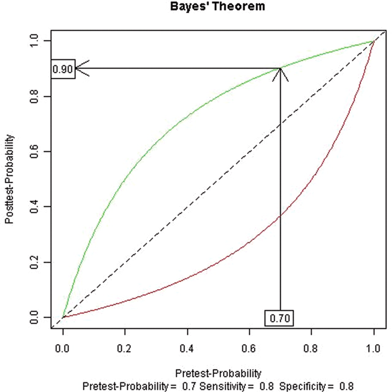
Using the above intuitive cut-offs, and tests with sensitivities and specificities between 80% and 90%, the above procedure is a good approximation to Bayes' theorem. A graphical approach to Bayes' theorem can demonstrate how the qualitative approximation works (figure 1). Here the horizontal-axis is the pretest probability, the curves represent the relationship between the pretest probability and the post-test probability for a given sensitivity and specificity (80% for each in this example, roughly corresponding to the test characteristics for a nuclear stress test) and the vertical-axis is the post-test probability. The diagonal line is usually included and represents no change in the post-test probability with the test result (ie, the test did not change the clinician's assessment of the probability). Separate curves represent a positive result (green), which increases the post-test probability (ie, is above the diagonal line), and a negative result (red), which reduces the post-test probability. To use Bayes' theorem, one starts on the horizontal-axis at the appropriate pretest probability and draws a vertical line until it intersects the appropriate curve for a positive (green) or negative test (red) result. One then draws a horizontal line to find the appropriate post-test probability on the vertical-axis. Figure 1 exemplifies this for the case above, a man with anginal chest pain and a positive stress test. One first locates 70% on the horizontal-axis, follows the arrow up until it intersects the positive result (green) curve, then follows the arrow horizontally until it intersects the vertical-axis at the post-test probability of 90%. A similar procedure is followed for a negative test, using the red line, giving a post-test probability of 37%.

• Download figure
• Open in new tab
• Download powerpoint

Figure 1

Graphical interpretation of Bayes' theorem.

In the categorical case, all the pretest probabilities between 67% and 90% (the likely category) need to be considered while holding the sensitivity and specificity constant at 80%. This only needs to be done for the lower (67%) and the upper limits (90%), see figure 2. For a positive test, the post-test probabilities range between 89% and 97% (arrows). To get the lower limit of post-test probability for a positive test, one follows the arrow from a pretest probability of 67% up until point A in figure 2 (where the arrow intersects the curve representing Bayes' theorem's post-test probability for a positive result), and then reads the post-test probability (89%) off the vertical-axis. For the upper limit of the post-test probability, one follows the arrow from a pretest probability of 90% up until point B in figure 2, and then finds the post-test probability (97%) on the vertical-axis. This gives the range of post-test probabilities for the likely category. For a negative result, the post-test probabilities range between 33% and 69%.

• Download figure
• Open in new tab
• Download powerpoint

Figure 2

Graphical interpretation of Bayes' theorem for a range of pretest probabilities from 67% to 90% (likely category).

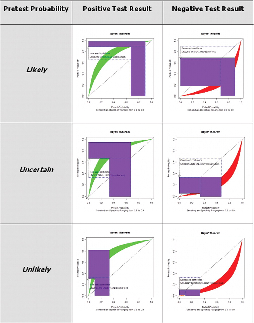
Next, expand the range of sensitivities and specificities from 80% to 90%, representing good tests. Now, instead of a (green) curve to represent the relationship between pretest and post-test probabilities, we have a (green) band (figure 3). Like before, one follows the arrow from the pretest probability until it firsts meets the band (A in figure 3) to get the lower limit of the post-test probability and until it meets the top of the band (B in figure 3) to get the upper limit of the post-test probability. For the likely category examined above, we can see that the post-test probabilities for a positive test now range between 89% and 99% – almost all in the very likely category – and for a negative test between 18% and 69% – almost all in the uncertain or unlikely categories. The transformation of the pretest probabilities is shown as the purple inverted ‘L’ in figure 3. The results for all the categories are shown in figure 4 and table 2.

• Download figure
• Open in new tab
• Download powerpoint

Figure 3

Graphical interpretation of Bayes' theorem for a range of pretest probabilities from 67% to 90% (likely category), and sensitivities and specificities ranging between 80% and 90%.

• Download figure
• Open in new tab
• Download powerpoint

Figure 4

Graphical interpretation of Bayes' theorem for a categorical probabilities, and sensitivities and specificities between 80% and 90%.

The method is an approximation. It forces a Bayesian inspired analysis on the interpretation of test results and gives results consistent with Bayes' theorem. The approximation is weakest in the two cells with contradictory data (eg, unlikely with a positive test result and likely with a negative test result) as expected. The results remain a good approximation even with expanded ranges for test characteristics (sensitivity and specificity). For example, if the range of test characteristics is between 70% and 80%, probability cut-offs of <20%, 20–45%, 46–55%, 56–80% and >80% work well. Since the method is only an approximation and our estimates of pretest probabilities are also poor estimates, just using the cut-offs likely, uncertain and unlikely will suffice.

Special cases

Rule-in and rule-out tests – tests in which a single result is capable of near definitively ruling-in or ruling-out a diagnosis – are important. For example, a low brain natriuretic peptide is suitable for ruling-out systolic heart failure. Any test with sensitivity greater than 99% is sufficient to rule-out a diagnosis from even the likely category (SnOUT) and any test with specificity greater than 99% is sufficient to rule-in a diagnosis from even the unlikely category (SpIN).

In the very categories, since the curves are fairly flat in this region (figure 1, for example), two tests might be needed to produce a clinically significant change in the probabilities.

This method does not apply to most screening tests because the pretest probabilities are so low. The method reminds the clinician that a positive result on a screening test is usually not diagnostic, because the change in probabilities is not large enough with a single test. It will usually take two tests to go from very unlikely (as target conditions are in the general population) to very likely (the final probability a clinician is interested in before undertaking a colectomy, mastectomy or prostatectomy). For example, a 45-year-old woman has a 5-year probability of having breast cancer of about 1%.11 The sensitivity of routine screening mammography ranges from 71% to 96% and the specificity ranges from 94% to 97%.12 Using values of 80% for sensitivity and 96% for specificity, a positive test increases the probability to 17%. Using the qualitative categories described herein, the woman's risk of breast cancer would go from very unlikely to unlikely with the single positive screening test.

Many diseases and tests have appropriate prevalences, and sensitivities and specificities for the tests published, for example, tropinin I for myocardial infarction13 or urine Chlamydia infection in men.14

Summary

In summary, here is a qualitative procedure to follow to approximate the results of a Bayesian diagnostic decision analysis.

1. What is the pretest probability of the disease being considered? Ideally this comes from an evidence-based source. If it is very likely (<10–20%) or very unlikely (>80–90%), in general, no further testing is needed.

2. One first categorises the pretest probability as likely, uncertain or unlikely.

3. If the test is positive, the post-test probability increases by one qualitative category (eg, unlikely to uncertain). If the test is negative, the post-test probability decreases by one qualitative category (eg, unlikely to very unlikely).

4. This process continues until the clinician is comfortable enough with the confidence in the diagnosis considering the patient's preferences, the risk of the disease and the effects of treatment.

5. Negative tests with sensitivities near 99% can almost certainly rule out a disease, since the post-test sensitivity will be very unlikely even if the original pretest probability was likely. Similarly, positive tests with specificities near 99% can almost certainly rule in a disease.

6. If the pretest probability was very likely or very unlikely, and further testing is indicated, two tests are needed to escape the very categories. This is because the change in the probabilities is small within these categories. Two concordant results are needed to change out of the very categories.